I find that Six Sigma and Design for Six Sigma courses are often eye-opening experiences for participants. There is an experience of discovering that there are tools available to answer problems that have vexed them, and learning that good engineering and science decisions can lead directly to good business outcomes through logical steps.
One of the most remarkable such moments is when students realize the importance of sample size. In the best cases, there is a forehead-slapping moment where the student realizes that much of the testing they’ve done in the past has probably been a complete waste of time; that while they thought they were seeing interesting differences and making good decisions, they were in fact only fooling themselves by comparing too-small data sets.
I want to show in the next few blog posts why sample size matters, both from a technical perspective and from a business perspective.
Design example
Throughout the next few posts, I’ll use the example of a manufactured product which the customer requires weigh at least 100 kg, sells for about $140 and that costs $120 to manufacture and convert to a sale (the cost of goods sold, or COGS, is $120).
| Sales |
|
140 |
| COGS |
|
120 |
| Material |
60 |
|
| Labor and Overhead |
60 |
|
| — |
— |
— |
| Gross Profit |
|
20 |
We want to develop a new version of the product, using a modified design and a new process that, by design, will reduce the cost of material by 10%. The old cost of material was 50% of COGS, or $60. To achieve the material cost reduction of 10%, we have to remove $6 in material costs, improving gross profit to $26.
We believe that the current design masses 120 kg, so we estimate that our new part mass should be  kg.
kg.
Seems like we might be done at this point, and I’ve seen plenty of engineering projects that stop here. Unfortunately, this isn’t the whole story. Manufacturing will be unable to produce parts of exactly 108 kg, so they’ll need a tolerance range to check parts against. We have that customer requirement for at least 100 kg, so any variation has to stay above that. We also want to save money relative to the current design, so we don’t want many parts to weigh much more than this, especially since the customer isn’t really willing to pay us for the “extra” material beyond 100 kg.
Population versus sample statistics
Most of process or product improvement is concerned with reducing the standard deviation,  , shifting the mean (a.k.a. average),
  , or reducing a proportion,
  , of a process or product characteristic. These summary statistics refer to the population characteristics—the mean, standard deviation or proportion of all parts of a certain design that will ever be produced, or all times that a production step will ever be completed in the intended manner.
Since we can’t measure the whole population up front—we will be producing parts for a long time—we have to draw a sample from the population, and use the statistics of that sample to gain insight into the total population. We can visualize this, somewhat crudely, with the following:
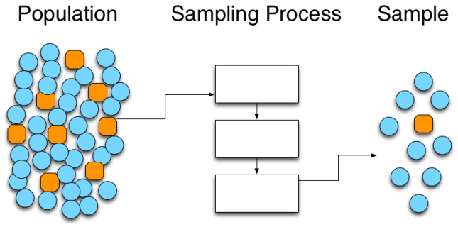
We can imagine that the blue circles are conforming parts, and the orange octagons are non-conforming parts. If the sampling process is fair, then the sample proportion  will be close to—and statistically indistinguishable from—the true population proportion . In the population we have 44 parts total, 8 defective parts and 36 conforming parts. In the sample that we drew, we have 10 parts total, 9 conforming and 1 defective. While
  , statistically we have
matrix(c(1, 8, 10-1, 44-8), ncol=2) %>%
  chisq.test(simulate.p.value = TRUE)
##
##  Pearson's Chi-squared test with simulated p-value (based on 2000
##  replicates)
##
## data:  matrix(c(1, 8, 10 - 1, 44 - 8), ncol = 2)
## X-squared = 0.3927, df = NA, p-value = 0.6692
With such a high p-value (0.67), we fail to reject the null hypothesis that  ; in more colloquial terms, we conclude that the apparent difference between 8/36 and 1/9 is only due to random errors in sampling. (For larger counts of successes and failures,
 prop.test() would also work and would be more informative.)
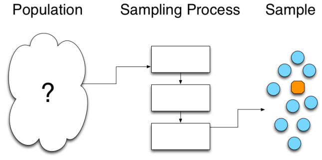
From our perspective, of course, we don’t know what the population looks like. We don’t have any way of knowing with certainty—or accessing data about—future performance, so there is no way for us to know what the total population looks like. In lieu of population data, we develop a sampling process that allows us to fairly draw a sample from that population.
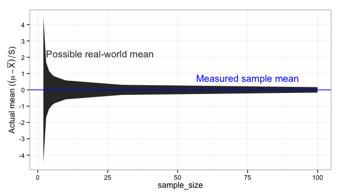
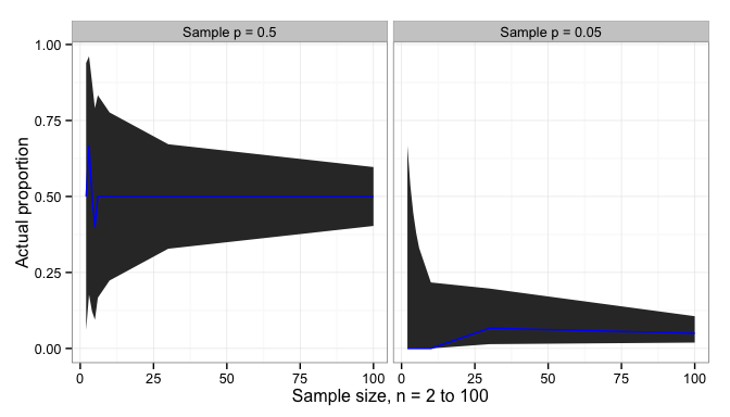
While we want to know the true population mean, , the true population standard deviation, , or the true population proportion , we can only calculate the sample mean,  , the sample standard deviation,
  , or the sample proportion .
From the known sample, we then reason backward to what the true population looks like. This is where statistics comes into play; statistics allows us to place rigorous boundaries on what the population may look like, without fooling ourselves. Sample size is critical to controlling the uncertainty in these boundaries.
Summary and a look forward
Testing in product development—and usually in production—involves sampling a product or process. Samples never look exactly like the population that we are concerned about, but if the sampling process is fair then the samples will be statistically indistinguishable from the population. With due awareness of the statistical uncertainties, we can use samples to make decisions about the population.
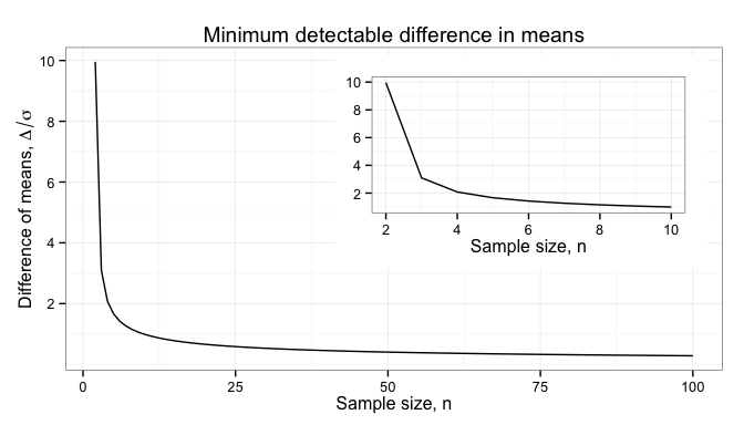
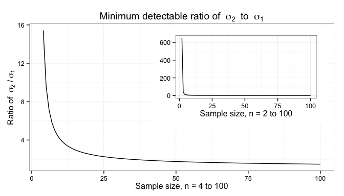
In the next post, I will look at how sample size impacts the uncertainty in our estimation of population statistics like the mean and standard deviation. In a later post, I will look at how this uncertainty impacts the business.
A short aside on statistical tests for proportions
The usual way to compare two proportions would be a proportions test (prop.test() in R), but because we have so few samples to compare, the results may be unreliable and prop.test() generates an appropriate warning. fisher.test() provides an exact estimate of the p-value, but the assumptions are violated with data like this, where we are sampling a fixed number of parts (i.e. row sums are fixed, but column sums are not controlled). This leaves us with using a chi-squared test (chisq.test() in R) which is less informative but does the job. Either the Barnard test or Bayesian estimation based on Monte Carlo simulation would be more informative and possibly more robust.


 , is proportional to the standard deviation of the sample,
 standard deviation.
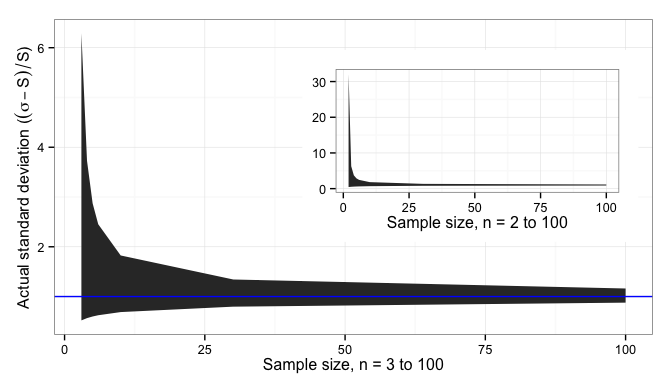


You must be logged in to post a comment.