Mean and sample size

The error in our estimate of the mean, , is proportional to the standard deviation of the sample, , and the sample size, .

We can visualize this easily enough by plotting the 95% confidence interval. When we sample and calculate the sample mean (), the true population mean, , (what we really want to know) is likely to be anywhere in the shaded region of the graph below.

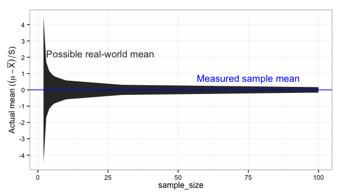
This graph shows the 95% confidence region for the true population mean, ; there’s a 95% chance that the true population mean is within this band. The “0” line on the y axis is our estimate of the mean, . We can’t know what the true population mean is, but it’s clear that if we use more samples, we can be sure that our estimate is closer to the true mean.

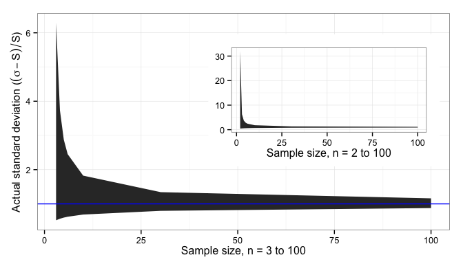
Standard deviation and sample size

Likewise, when we calculate the sample standard deviation, , the true standard deviation, has a 95% chance of being within the confidence band below. For small sample sizes (roughly less than 10), the measured standard deviation can be off from the true standard deviation by several times. Even for ten samples, the potential error is nearly standard deviation.

Proportion and sample size

For proportions, the situation is similar: there is a 95% chance that the true sample proportion, , is within the shaded band based on the measured sample proportion . Since this confidence interval depends on and cannot be standardized the way and can be, confidence intervals for two different proportions are plotted.

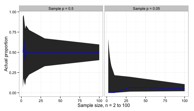
For small , proportions data tells us very little.

Process capability and production costs

The cost of poor quality in product or process design can be characterized by the Cpk:

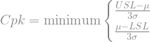
Where USL is the upper specification limit (also called the upper tolerance) and LSL is the lower specification limit (or lower tolerance).

We can estimate the defect rate (defects per opportunity, or DPO) from the Cpk:

That probability function is calculated in R with pnorm(3 * Cpk - 1.5) and in Excel with NORMSDIST(3 * Cpk - 1.5). The 1.5 is a typical value used to account for uncorrected or undetected process drift.

Since we don’t know and , we have to substitute and . The uncertainty in these estimates of the population and mean that we have uncertainty in what the true process Cpk (or defect rates) will be once we’re in production. When our sample testing tells us that the Cpk should be 1.67 (the blue line), the true process Cpk will actually turn out to be somewhere in the shaded band:

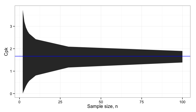
Below the blue line, our product or process is failing to meet customer expectations, and will result in lost customers or higher warranty costs. Above the blue line, we’ve added more cost to the production of the product than we need to, reducing our gross profit margin. Since that gray band doesn’t completely disappear, even at 100 samples, we can never eliminate these risks; we have to find a way to manage them effectively.

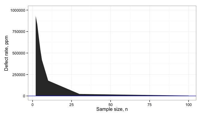
The impact of this may be more evident when we convert from Cpk to defect rates (ppm):

Summary and a look forward

With a fair sampling process, samples will look similar to—and statistically indistinguishable from—the population that they were drawn from. How much they look like the population depends critically on how many samples are tested. The uncertainties, or errors in our estimates, resulting from sample size decisions have impacts all through our design analysis and production planning.

In the next post, I will explore in more detail how these uncertainties impact our experiment designs.