We’ve seen in the previous posts that in designing products we need to know characteristics like the mean and standard deviation of the population, but are limited to only being able to measure sample means and standard deviations. This leaves us with uncertainty in our knowledge of population characteristics, and that uncertainty directly impacts our ability to make better products. In this post, we’ll see how business financial requirements and estimation uncertainties due to sample size interact both to to further limit our available design options and to drive up our sample size requirements.
Impact on specifications
Looking back at our graph of Cpk, Cpk values below the target value (blue line) increase production and sales costs through increased rework, scrap and warranty. Above the blue line, we’ve added product or production costs by over-designing the product or process. Since the price of a product is determined by the market, any increase in cost decreases our gross profit margin:

As outlined in the first post of this series, we are going to cut material costs by 10% on a part that had to weigh at least 100 kg. That was a $6 reduction in costs on a $120 part.
Our first issue is that we have to be sure that we have a good baseline for improvement. If the existing parts are very different than our expectations, we may be creating more trouble by making changes. We also don’t know how much variation there is in part weight.
We collect production data over a week and determine that the current mean part weight is, as expected, 120 kg with a standard deviation of 6.7 kg. With 120 kg of material, we calculate a Cpk of

We calculate that we have to remove 
Any single product below 100 kg runs the risk of being rejected by the customer, possibly at great cost (e.g. they may require special field service on older parts, or decide to buy from a competitor in the future, or both), so we don’t want to have a higher defect rate with the new product and process than with the old, because this will increase labor and overhead costs. With the new product and process, we want to target a standard deviation of at least
We might stop there, and say that when we have a design for 108 kg and prototypes that weigh on average 108 kg with a standard deviation of up to 2.7 kg, we’re done. Our specification now looks like this:
| Minimum | Maximum | Target | |
|---|---|---|---|
| Part Weight | 100 | 108 | ? |
| Standard Deviation | 0 | 2.7 | ? |
| Cpk | 1.0 | ? | ? |
However, there would be substantial risk that we would not achieve our goals of both meeting the customer requirement of 100 kg and reducing material costs by 10%. Using these numbers as our target, we have a 50% chance that we will be over the cost target, and a 50% chance that our defect rate will be higher than target.
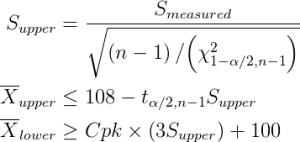
In order to meet customer requirements, we want to be confident that all parts weigh at least 100 kg. In order to meet business needs, we have to be 95% confident that at least half of our product weighs at most 108 kg.
For the customer requirement, we need to calculate the Cpk. In the past, “all” product really meant a Cpk of 1.0, or 93% of product. To calculate this we need our 95% confidence estimate of the mean, 

For the business requirement, we need the confidence bounds on our estimate of the mean,

Now we need to design and build our prototypes. How many parts do we build and weigh? Recognizing that there will be uncertainty in our estimate of 


We have to use the confidence bounds on
These equations are easier to understand if we graph them for several values of
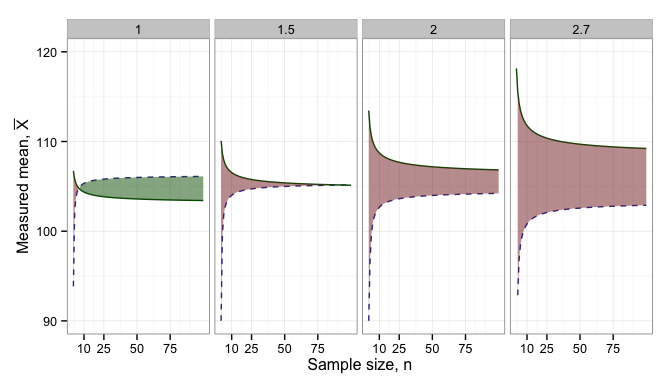
This graph shows the maximum and minimum possible
As can be seen, while we calculated a naive target for standard deviation,
We can now ammend our requirements:
| Minimum | Maximum | Target | |
|---|---|---|---|
| Part Weight | 100 | 108 | 105.5 |
| Standard Deviation | 0 | 2.7 | (from Cpk) |
| Cpk | 1.0 | f(n, S) | 1.0 |
|
f(n, S) | f(n, S) | 104 |
|
0 | 1.2 | 1.0 |
| n (for sampling) | 10 | 100 | 10 |
Not only do we have to design our product and process to be more stringent than the naive requirements, we have to test more than we might otherwise wish to.
Importantly, our specification now contains the tolerance ranges on the weight, the standard deviation of the weight, and the Cpk. This is the minimum set of information that we need to fully specify a part. For the purposes of testing and checking short-term process performance, we also need to specify the number of samples to collect and sample mean and standard deviation.
UPDATE 2016-08-25: Equations were no longer rendering correctly; this was fixed.
References
- R Core Team (2014). R: A language and environment for statistical computing. R Foundation for Statistical Computing, Vienna, Austria. URL http://www.R-project.org/.
- H. Wickham. ggplot2: elegant graphics for data analysis. Springer New York, 2009.
