Update to plot.qcc using ggplot2 and grid

Two years ago, I blogged about my experience rewriting the plot.qcc() function in the qcc package to use ggplot2 and grid. My goal was to allow manipulation of qcc’s quality control plots using grid graphics, especially to combine range charts with their associated individuals or moving range charts, as these two diagnostic tools should be used together. At the time, I posted the code on my GitHub.

I recently discovered that the update to ggplot2 v2.0 broke my code, so that attempting to generate a qcc plot would throw an obscure error from someplace deep in ggplot2. The fix turned out to be pretty easy. The original code used aes_string() instead of aes() because of a barely-documented problem of calling aes() inside a function. It looks like this has been quietly corrected with ggplot2 2.0, and aes_string() is no longer needed for this.

The updated code is up on GitHub. As before, load the qcc library, then source() qcc.plot.R. For the rest of the current session, calls to qcc() will automatically use the new plot.qcc() function.

Normality and Testing for Normality

Many of our statistical tests make assumptions about the distribution of the underlying population. Many of the most common—ImR (XmR) and XbarR control charts, ANOVA, t-tests—assume normal distributions in the underlying population (or normal distributions in the residuals, in the case of ANOVA), and we’re often told that we must carefully check the assumptions.

At the same time, there’s a lot of conflicting advice about how to test for normality. There are the statistical tests for normality, such as Shapiro-Wilk or Anderson-Darling. There’s the “fat pencil” test, where we just eye-ball the distribution and use our best judgement. We could even use control charts, as they’re designed to detect deviations from the expected distribution. We are discouraged from using the “fat pencil” because it will result in a lot of variation from person to person. We’re often told not to rely too heavily on the statistical tests because they are not sensitive with small sample sizes and too sensitive to the tails. In industrial settings, our data is often messy, and the tails are likely to be the least reliable portion of our data.

I’d like to explore what the above objections really look like. I’ll use R to generate some fake data based on the normal distribution and the t distribution, and compare the frequency of p-values obtained from the Shapiro-Wilk test for normality.

A Function to test normality many times

First, we need to load our libraries

library(ggplot2)
library(reshape2)

To make this easy to run, I’ll create a function to perform a large number of normality tests (Shapiro-Wilk) for sample sizes n = 5, 10 and 1000, all drawn from the same data:

#' @name assign_vector
#' @param data A vector of data to perform the t-test on.
#' @param n An integer indicating the number of t-tests to perform. Default is 1000
#' @return A data frame in "tall" format
assign_vector <- function(data, n = 1000) {
  # replicate the call to shapiro.test n times to build up a vector of p-values
  p.5 <- replicate(n=n, expr=shapiro.test(sample(my.data, 5, replace=TRUE))$p.value)
  p.10 <- replicate(n=n, expr=shapiro.test(sample(my.data, 10, replace=TRUE))$p.value)
  p.1000 <- replicate(n=n, expr=shapiro.test(sample(my.data, 1000, replace=TRUE))$p.value)
  #' Combine the data into a data frame, 
  #' one column for each number of samples tested.
  p.df <- cbind(p.5, p.10, p.1000)
  p.df <- as.data.frame(p.df)
  colnames(p.df) <- c("5 samples","10 samples","1000 samples")
  #' Put the data in "tall" format, one column for number of samples
  #' and one column for the p-value.
  p.df.m <- melt(p.df)
  #' Make sure the levels are sorted correctly.
  p.df.m <- transform(p.df.m, variable = factor(variable, levels = c("5 samples","10 samples","1000 samples")))
  return(p.df.m)  
}

Clean, random data

I want to simulate real-word conditions, where we have an underlying population from which we sample a limited number of times. To start, I’ll generate 100000 values from a normal distribution. To keep runtimes low I’ll have assign_vector() sample from that distribution when performing the test for normality.

n.rand <- 100000
n.test <- 10000
my.data <- rnorm(n.rand)
p.df.m <- assign_vector(my.data, n = n.test)

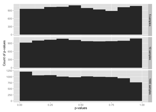
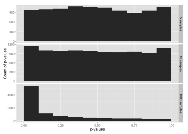
We would expect that normally distributed random data will have an equal probability of any given p-value. i.e. 5% of the time we’ll see p-value ≤ 0.05, 5% of the time we’ll see p-value > 0.05 and ≤ 0.10, and so on through > 0.95 and ≤ 1.00. Let’s graph that and see what we get for each sample size:

ggplot(p.df.m, aes(x = value)) + 
  geom_histogram(binwidth = 1/10) + 
  facet_grid(facets=variable ~ ., scales="free_y") + 
  xlim(0,1) +
  ylab("Count of p-values") +
  xlab("p-values") +
  theme(text = element_text(size = 16))

Histogram of p-values for the normal distribution, for sample sizes 5, 10 and 1000.

This is, indeed, what we expected.

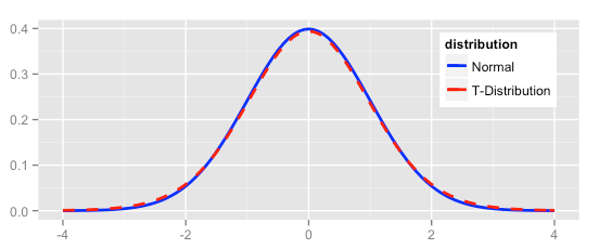
Now let’s compare the normal distribution to a t distribution. The t distribution would pass the “fat pencil” test—it looks normal to the eye:

ggplot(NULL, aes(x=x, colour = distribution)) + 
  stat_function(fun=dnorm, data = data.frame(x = c(-6,6), distribution = factor(1)), size = 1) + 
  stat_function(fun=dt, args = list( df = 20), data = data.frame(x = c(-6,6), distribution = factor(2)), linetype = "dashed", size = 1) + 
  scale_colour_manual(values = c("blue","red"), labels = c("Normal","T-Distribution")) +
  theme(text = element_text(size = 12),
        legend.position = c(0.85, 0.75)) +
  xlim(-4, 4) +
  xlab(NULL) +
  ylab(NULL)

Starting with random data generated from the t-distribution:

my.data <- rt(n.rand, df = 20)

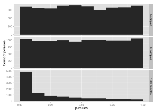
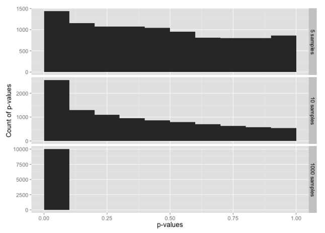
Histogram of p-values for the t distribution, for sample sizes 5, 10 and 1000.

The tests for normality are not very sensitive for small sample sizes, and are much more sensitive for large sample sizes. Even with a sample size of 1000, the data from a t distribution only fails the test for normality about 50% of the time (add up the frequencies for p-value > 0.05 to see this).

Testing the tails

Since the t distribution is narrower in the middle range and has longer tails than the normal distribution, the normality test might be failing because the entire distribution doesn’t look quite normal; we haven’t learned anything specifically about the tails.

To test the tails, we can construct a data set that uses the t distribution for the middle 99% of the data, and the normal distribution for the tails.

my.data <- rt(n.rand, df = 20)
my.data.2 <- rnorm(n.rand)
# Trim off the tails
my.data <- my.data[which(my.data < 3 & my.data > -3)]
# Add in tails from the other distribution
my.data <- c(my.data, my.data.2[which(my.data.2 < -3 | my.data.2 > 3)])

Histogram of p-values for sample sizes 5, 10 and 1000, from a data set constructed from the t distribution in the range -3 to +3 sigmas, with tails from the normal distribution below -3 and above +3.

Despite 99% of the data being from the t distribution, this is almost identical to our test with data from just the normal distribution. It looks like the tails may be having a larger impact on the normality test than rest of the data

Now let’s flip this around: data that is 99% normally-distributed, but using the t distribution in the extreme tails.

my.data <- rnorm(n.rand)
my.data.2 <- rt(n.rand, df = 20)
# Trim off the tails
my.data <- my.data[which(my.data < 3 & my.data > -3)]
# Add in tails from the other distribution
my.data <- c(my.data, my.data.2[which(my.data.2 < -3 | my.data.2 > 3)])

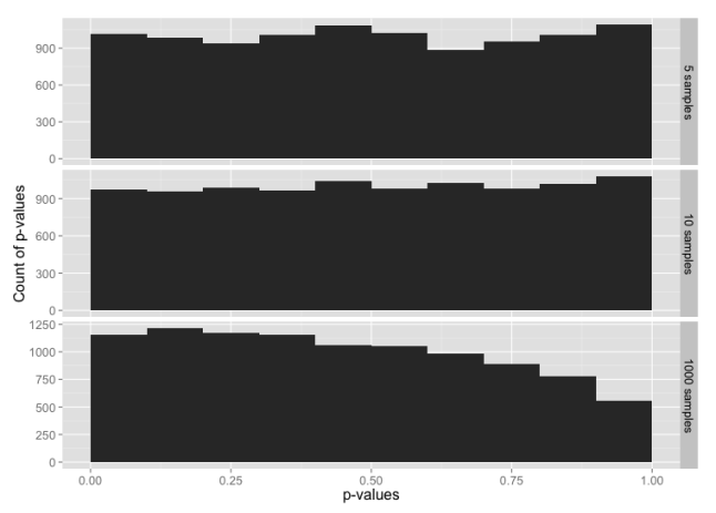
Histogram of p-values for sample sizes 5, 10 and 1000, from a data set constructed from the normal distribution in the range -3 to +3 sigmas, with tails from the t-distribution below -3 and above +3.

Here, 99% of the data is from the normal distribution, yet the normality test looks almost the same as the normality test for just the t-distribution. If you check the y-axis scales carefully, you’ll see that the chance of getting p-value ≤ 0.05 is a bit lower here than for the t distribution.

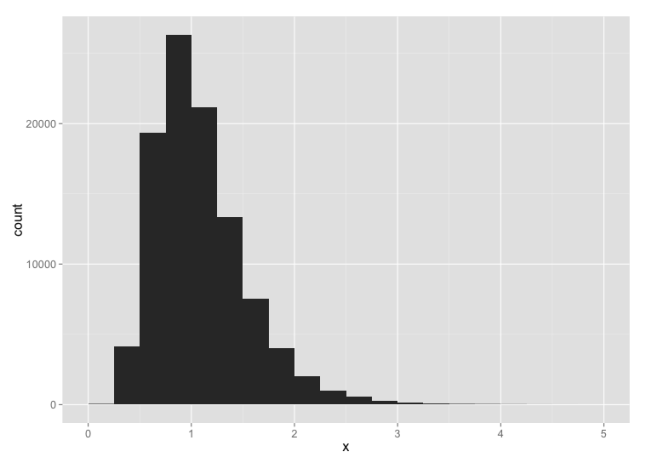
To make the point further, suppose we have highly skewed data:

my.data <- rlnorm(n.rand, 0, 0.4)

This looks like:

For small sample sizes, even this is likely to pass a test for normality:

What have we learned?

With small sample sizes, everything looks normal.
The normality tests are, indeed, very sensitive to what goes on in the extreme tails.

In other words, if we have enough data to fail a normality test, we always will because our real-world data won’t be clean enough. If we don’t have enough data to reliably fail a normality test, then there’s no point in performing the test, and we have to rely on the fat pencil test or our own understanding of the underlying processes.

Don’t get too hung up on whether your data is normally distributed or not. When evaluating and summarizing data, rely mainly on your brain and use the statistics only to catch really big errors in judgement. When attempting to make predictions about future performance, e.g. calculating Cpk or simulating a process, recognize the opportunities for errors in judgment and explicitly state you assumptions.

Rewriting plot.qcc using ggplot2 and grid

The free and open-source R statistics package is a great tool for data analysis. The free add-on package qcc provides a wide array of statistical process control charts and other quality tools, which can be used for monitoring and controlling industrial processes, business processes or data collection processes. It’s a great package and highly customizable, but the one feature I wanted was the ability to manipulate the control charts within the grid graphics system, and that turned out to be not so easy.

I went all-in and completely rewrote qcc’s plot.qcc() function to use Hadley Wickham’s ggplot2 package, which itself is built on top of grid graphics. I have tested the new code against all the examples provided on the qcc help page, and the new ggplot2 version works for all the plots, including X-bar and R, p- and u- and c-charts.

In qcc, an individuals and moving range (XmR or ImR) chart can be created simply:

library(qcc)
my.xmr.raw <- c(5045,4350,4350,3975,4290,4430,4485,4285,3980,3925,3645,3760,3300,3685,3463,5200)
x <- qcc(my.xmr.raw, type = "xbar.one", title = "Individuals Chart\nfor Wheeler sample data")
x <- qcc(matrix(cbind(my.xmr.raw[1:length(my.xmr.raw)-1], my.xmr.raw[2:length(my.xmr.raw)]), ncol = 2), type = "R", title = "Moving Range Chart\nfor Wheeler sample data")

This both generates the plot and creates a qcc object, assigning it to the variable x. You can generate another copy of the plot with plot(x).

To use my new plot function, you will need to have the packages ggplot2, gtable, qcc and grid installed. Download my code from the qcc_ggplot project on Github, load qcc in R and then run source("qcc.plot.R"). The ggplot2-based version of the plotting function will be used whenever a qcc object is plotted.

library(qcc)
source("qcc.plot.R")
my.xmr.raw <- c(5045,4350,4350,3975,4290,4430,4485,4285,3980,3925,3645,3760,3300,3685,3463,5200)
x <- qcc(my.xmr.raw, type = "xbar.one", title = "Individuals Chart\nfor Wheeler sample data")
x <- qcc(matrix(cbind(my.xmr.raw[1:length(my.xmr.raw)-1], my.xmr.raw[2:length(my.xmr.raw)]), ncol = 2), type = "R", title = "Moving Range Chart\nfor Wheeler sample data")

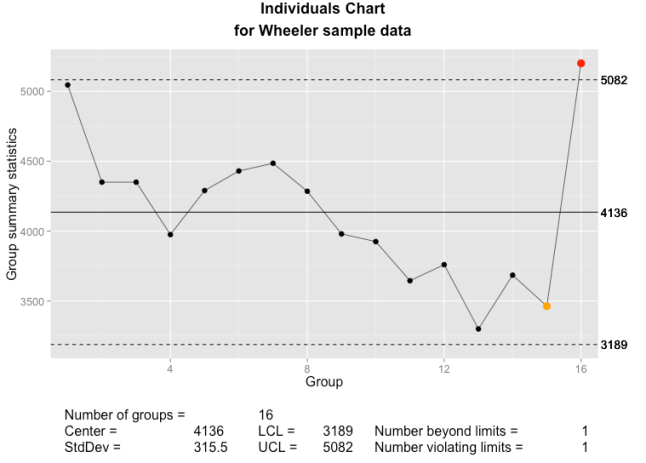
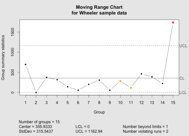
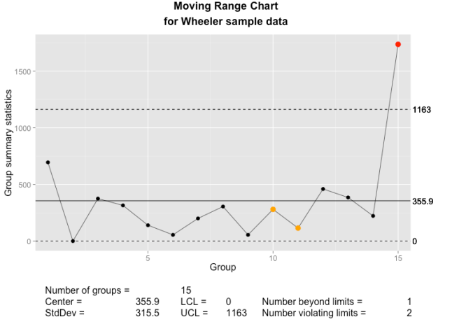
Below, you can compare the individuals and moving range charts generated by qcc and by my new implementation of plot.qcc():

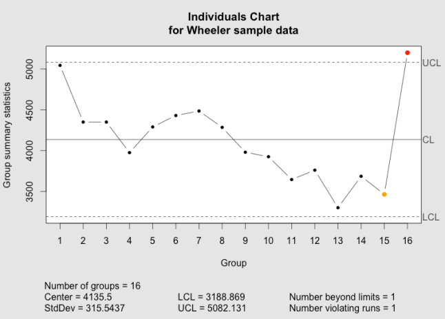
The qcc individuals chart as implemented in the qcc package.

The qcc individuals chart as implemented using ggplot2 and grid graphics.

The qcc moving range chart as implemented in the qcc package.

The qcc moving range chart as implemented using ggplot2 and grid graphics.

New features

In addition to the standard features in qcc plots, I’ve added a few new options.

size or cex: Set the size of the points used in the plot. This is passed directly to geom_point().
font.size: Sets the size of text elements. Passed directly to ggplot() and grid’s viewport().
title = element_blank(): Eliminate the main graph title completely, and expand the data region to fill the empty space. As with qcc, with the default title = NULL a title will be created, or a user-defined text string may be passed to title.
new.plot: If TRUE, creates a new graph (grid.newpage()). Otherwise, will write into the existing device and viewport. Intended to simplify the creation of multi-panel or composite charts.
digits: The argument digits is provided by the qcc package to control the number of digits printed on the graph, where it either uses the default option set for R or a user-supplied value. I have tried to add some intelligence to calculating a default value under the assumption that we can tell something about the measurement from the data supplied. You can see the results in the sample graphs above.

Lessons Learned

This little project turned out to be somewhat more difficult than I had envisioned, and there are several lessons-learned, particularly in the use of ggplot2.

First, ggplot2 really needs data frames when plotting. Passing discrete values or variables not connected to a data frame will often result in errors or just incorrect results. This is different than either base graphics or grid graphics, and while Hadley Wickham has mentioned this before, I hadn’t fully appreciated it. For instance, this doesn’t work very well:

my.test.data <- data.frame(x = seq(1:10), y = round(runif(10, 100, 300)))
my.test.gplot <- ggplot(my.test.data, aes(x = x, y = y)) + 
  geom_point(shape = 20)
index.1 <- c(5, 6, 7)
my.test.gplot <- my.test.gplot +
  geom_point(aes(x = x[index.1], y = y[index.1]), col = "red")
my.test.gplot

Different variations of this sometimes worked, or sometimes only plotted some of the points that are supposed to be colored red.

However, if I wrap that index.1 into a data frame, it works perfectly:

my.test.data <- data.frame(x = seq(1:10), y = round(runif(10, 100, 300)))
my.test.gplot <- ggplot(my.test.data, aes(x = x, y = y)) + 
  geom_point(shape = 20)
index.1 <- c(5, 6, 7)
my.test.subdata <- my.test.data[index.1,]
my.test.gplot <- my.test.gplot +
  geom_point(data = my.test.subdata, aes(x = x, y = y), col = "red")
my.test.gplot

Another nice lesson was that aes() doesn’t always work properly when ggplot2 is called from within a function. In this case, aes_string() usually works. There’s less documentation than I would like on this, but you can search the ggplot2 Google Group or Stack Overflow for more information.

One of the bigger surprises was discovering that aes() searches for data frames in the global environment. When ggplot() is used from within a function, though, any variables created within that function are not accessible in the global environment. The work-around is to tell ggplot which environment to search in, and a simple addition of environment = environment() within the ggplot() call seems to do the trick. This is captured in a stack overflow post and the ggplot2 issue log.

my.test.data <- data.frame(x = seq(1:10), y = round(runif(10, 100, 300)))
my.test.gplot <- ggplot(my.test.data, environment = environment(), aes(x = x, y = y)) + 
  geom_point(shape = 20)
index.1 <- c(5, 6, 7)
my.test.subdata <- my.test.data[index.1,]
my.test.gplot <- my.test.gplot +
  geom_point(data = my.test.subdata, aes(x = x, y = y), col = "blue")
my.test.gplot

Finally, it is possible to completely and seamlessly replace a function created in a package and loaded in that package’s namespace. When I set out, I wanted to end up with a complete replacement for qcc’s internal plot.qcc() function, but wasn’t quite sure this would be possible. Luckily, the below code, called after the function declaration, worked. One thing I found was that I needed to name my function the same as the one in the qcc package in order for the replacement to work in all cases. If I used a different name for my function, it would work when I called plot() with a qcc object, but qcc’s base graphics version would be used when calling qcc() with the parameter plot = TRUE.

unlockBinding(sym="plot.qcc", env=getNamespace("qcc"));
assignInNamespace(x="plot.qcc", value=plot.qcc, ns=asNamespace("qcc"), envir=getNamespace("qcc"));
assign("plot.qcc", plot.qcc, envir=getNamespace("qcc"));
lockBinding(sym="plot.qcc", env=getNamespace("qcc"));

Outlook

For now, the code suits my immediate needs, and I hope that you will find it useful. I have some ideas for additional features that I may implement in the future. There are some parts of the code that can and should be further cleaned up, and I’ll tweak the code as needed. I am certainly interested in any bug reports and in seeing any forks; good ideas are always welcome.

References

R Core Team (2013). R: A language and environment for statistical computing. R Foundation for Statistical Computing, Vienna, Austria. URL http://www.R-project.org/.
Scrucca, L. (2004). qcc: an R package for quality control charting and statistical process control. R News 4/1, 11-17.
H. Wickham. ggplot2: elegant graphics for data analysis. Springer New York, 2009.
Wheeler, Donald. “Individual Charts Done Right and Wrong.” Quality Digest. 2 Feb 20102 Feb 2010. Print. <http://www.spcpress.com/pdf/DJW206.pdf>.

Tom Hopper

Competitive organizations through high-performance learning

statistical process control